Table of Contents
- Note
- The example is based on the Diploma thesis "Effiziente, approximative Berechnung des Spektrums von Graphen mittels hierarchischer Matrizen" by Jan Nitzschmann.
Problem Description
Given is a Graph \(G = (V,E)\) with nodes \(V = \left\{v_1,\ldots,v_n\right\}\) and edges \(E \subseteq V \times V\). Let \(\mathcal{L} := I - D^{-1/2} A D^{-1/2}\) be the normalised Laplacian of \(G\) with diagonal \(D, d_{ii} := \textrm{degree}(v_i)\), and adjacency matrix \(A\),
\[ a_{ij} := \left\{ \begin{array}{ll} 1 & (i,j) \in E \\ 0 & \textrm{otherwise} \end{array} . \right. \]
We are looking for the spectrum \(\Lambda = \left\{ \lambda_1, \ldots, \lambda_n \right\} \) of \(\mathcal{L}\). Please note, that \(\Lambda \subset [0,2]\) with \(\lambda_1 = 0\).
Computing all eigenvalues \(\lambda_i\) is usually extremly costly. However, sometimes not the exact spectrum is of interest but the general distribution of eigenvalues, which permits to characterise certain properties of matrices and especially graphs.
Applying the convolution
\[ f_{\mu}(\lambda_0) := \sum_{\lambda_i} \int k_{\mu}(\lambda_0,\lambda') \delta(\lambda' - \lambda_i) d\lambda' \]
with
\[ k_{\mu}(\lambda_0,\lambda') := \frac{\mu}{(\lambda' - \lambda_0)^2 + \mu^2} \]
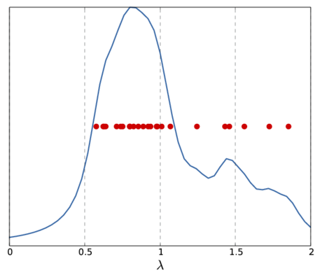
and \(\delta\) being the usual delta distribution, one obtains a graphical representation of the spectrum. An example for this is shown in the following picture for a small graph (left) and the convoluted spectrum of its Laplacian together with the eigenvalues.
 |  |
| Graph | Spectrum |
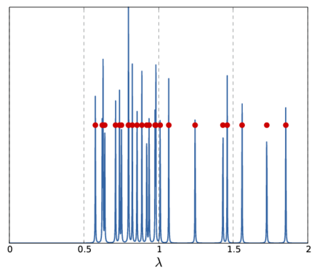
Note, that the above \(f_{\mu}(\lambda_0)\) only represents a single sample for the whole spectrum. Depending on the sample frequency and the choice of \(\mu\), the final image shows more or less details of the spectrum. The following picture show two other versions of the above spectrum with a coarse (left) and fine (right) sampling.
 |  |
Computation of the Spectrum
The above definition of \(f_{\mu}(\lambda_0)\) contains the eigenvalues, which are not available. Hence, another way to compute \(f_{\mu}(\lambda_0)\) is needed.
We start with the computation of the determinant of \(\mathcal{L}-\lambda I\) using LU factorisation. Since the determinant of triangular matrices is the product of their diagonal entries and since the diagonal entries of \(L\) are one, this can be restricted to the diagonal entries of \(U\):
\[ |\textrm{det}(\mathcal{L}-\lambda I)| = |\textrm{det}(LU)| = |\textrm{det}(U)| = |\prod_i u_{ii}|. \]
Applying the logarithm to both sides of the equation, we can change the product into a sum:
\[ \log |\textrm{det}(\mathcal{L}-\lambda I)| = \log |\prod_i u_{ii}| = \sum_i \log |u_{ii}|. \]
Replacing \(\lambda\) by \(\lambda_0 + i\mu\), one obtains
\begin{eqnarray*} \sum_i \log |u_{ii}| & = & \log |\textrm{det}(\mathcal{L}-(\lambda_0 + i\mu) I)| \\ & = & \log \prod_{\lambda_i} |\lambda_i - \lambda_0 - i\mu| \\ & = & \sum_{\lambda_i} \log |\lambda_i - \lambda_0 - i\mu| \end{eqnarray*}
Here we have used the identity of the determinant with the corresponding characteristic polynomial \(\prod_{\lambda_i} (\lambda_i - *)\).
Finally, differentiation with respect to \(\mu\) yields
\begin{eqnarray*} \frac{d}{d\mu} \sum_i \log |u_{ii}| & = & \sum_{\lambda_i} \frac{d}{d\mu} \log |\lambda_i - \lambda_0 - i\mu| \\ & = & \sum_{\lambda_i} \frac{d}{d\mu} \frac{1}{2} \log | (\lambda_i - \lambda_0)^2 + \mu^2| \\ & = & \sum_{\lambda_i} \frac{\mu}{(\lambda_i - \lambda_0)^2 + \mu^2} \\ & = & f_{\mu}(\lambda_0). \end{eqnarray*}
Replacing the differentation by a (central) difference quotient makes the problem computable with a series of LU factorisations for \(\mathcal{L}-(\lambda_0+i\mu)I\) for the different values of \(\lambda_0\). Furthermore, instead of an exact LU decomposition, the H-LU factorisation is used to maintain log-linear costs.
Sparse to H-Matrix Conversion
The program starts by converting a sparse matrix, which is assumed to represent a graph laplacian, into an H-matrix:
In addition to \(L\) also the identity matrix is needed to compute \(\mathcal{L}-(\lambda_0+i\mu)I\):
Both matrices need to be complex valued since \(\lambda_0+i\mu\) is, except for \(\mu = 0\), represents the limit case with exact representation of the spectrum. Therefore the value type was chosen be complexed valued.
Computing the Difference Quotient
For the computation of the spectrum in the sample space \([0,2]\) equally distant sample points are chosen as defined by the number of steps nsteps, i.e., \(\lambda_0 = 0, h_s, 2 \cdot h_s, ..., 2\) with \(h_s = 2/\textrm{nsteps}\).
Afterwards, for each value of \(\lambda_0\) the difference quotient is computed and \(\lambda_0\) as well as the result of the difference quotient are stored:
Since computation for different values of \(\lambda_0\) are independent, they may be computed in parallel. This is done by using the parallel_for algorithm from TBB:
- Remarks
- Although H-LU scales very good with the number of cores, it is even more efficient to perform factorisations in parallel since there are still some portions of the algorithm implemented sequentially.
The result of the computation is stored in two objects of type BLAS::Vector and returned as a std::pair, which completes the function calc_y:
This is then called from the main function via
For visualization, both arrays are written to files in Matlab format, which finishes the program:
Computing the Determinant
Left open is the computation of the determinant of \(\mathcal{L}-(\lambda_0+i\mu)I\) implemented in calc_abs_det via H-LU factorisation.
Before the factorisation, the matrix first has to be computed:
By default, 𝖧𝖫𝖨𝖡𝗉𝗋𝗈 uses block-wise LU factorisation, i.e., computes the inverse of diagonal blocks. In this case however, the point-wise LU factorisation is needed since the diagonal entries are used.
After the factorisation, these diagonal entries only need to be extracted from the matrix. Note, that L_lmu_id stores \(L\) and \(U\) but since the diagonal entries of \(L\) are one and therefore not explicitly stored, the diagonal of L_lmu_id is equal to the diagonal of \(U\).
To obtain the diagonal entries the function diagonal is available, which returns a vector containing the coefficients.
In order to prevent stability issues, the function tests for very small values and aborts further computation if such values are present:
The Plain Program
Example Matrices
The Sparse Matrix Collection from the University of Florida provides a wide range of sparse matrices.
The following Matlab function will compute the normalised Laplacian from a given sparse matrix, assuming the matrix contains the adjacency matrix of the graph (loops are ignored!).